| Table of Contents |
|---|
Overview of the Solargis
...
APIs
The purpose of the Solargis API is to provide automated access to Solargis data and services for computers over the web. API is the "user interface" for developers. Developers can automate integrating Solargis products into customized solutions. Table: overview of data available through the Solargis API.
| Availability of PV, solar and meteorological data | Technical features | ||||||
historical | operational | real-time and nowcasting | ||||||
|---|---|---|---|---|---|---|---|---|
numerical weather forecasting | long-term average | type of communication | request type |
|---|
response type | ||||||||
|---|---|---|---|---|---|---|---|---|
Data Delivery Web Service | YES | YES | YES | YES | NO | synchronous over HTTPS | XML | XML |
LTA Web Service (LTA API) | NO | NO | NO | NO | YES | synchronous over HTTPS | XML | XML |
Push data delivery | YES | YES | YES | YES | NO | regular push to SFTP scheduled |
by Solargis |
CSV | CSV |
Solargis web services consist of two different endpoints:
Data Delivery Web Service - the main service for accessing Solargis time series data. Both request and response is an are XML documentdocuments. The request parameters (XML elements and attributes) are formally described by based on the XML Schema Definition documents (XSD). By using the schema, request or response can be verified programmatically. For this service, we provide two endpoints - the REST-like endpoint, and the SOAP endpoint. Look for more technical information here. Authentication and billing is based on API key registered with the user. Please contact us to discuss details, set up trial or ask for a quotation.
LTA Web Service - this a simple web service provides monthly long-term averaged data (including also the yearly value) of PV, solar and meteorological data with global coverage. The service is aimed for automation of prospection and pre-feasibility . By sending an XML request the user mimics the click on the Calculate button in the interactive Solargis Prospect application. Request and response for the service is not described in this user guideof PV projects. More information can be found here.
Additionally, we provide the Push data delivery service where the request (a CSV file) is stored in the user's remote directory (SFTP, Azure, ...S3). The service is then scheduled to push CSV response data files regularly . Request processing is asynchronous - the client uploads the CSV request, the server processes the request according to a schedule ( e.g., once a day , or every hour), the client then checks for the response files. The . The CSV request allows for multiple locations in one a single file. For pricing and setting up a trial FTP user account, please contact us.
In the case of the solar and PV time series, we use satellite data since available history up to the present moment plus additional nowcasting for additional 5 hours ahead. The range of the satellite data includes historical / (archived) data, operational data, real-time data and the Cloud Motion Vector model (CMV, also called as nowcasting). Historical data ranges up to the last completed calendar month and can be considered as "definitive". Data in the current calendar month up to DAY-1 is so-called "operational", and will be re-analyzed in the beginning of the next month using the final version of required data inputs. Important is to note that differences introduced with the re-analysis are typically small. Solar data in the current day comes from the "real-time" satellite data and will be updated as soon as the current day is finished. Then, based on the latest satellite images, we predict solar data parameters by using the CMV model in the range of next 5 hours. The present moment and a short period before is covered by the nowcasting data as the very recent satellite scene is still in progress. This delay can take up to 30 minutes (depending on the satellite scanning frequency). Later on, after the nowcasting time range, we use post-processed output from Numerical Weather Prediction models (NWP). Satellite-based data is seamlessly integrated with the NWP data within the response. In the case of locations where satellite real-time & nowcasting data is not yet available, the NWP data is used over the course of the current day. All meteorological data (TEMP, WS, AP, RH,...) comes come from the NWP data sources.
The schema below shows how the data sources are integrated into the response.
...
Satellite based solar data
...
Spatial availability of the satellite data
...
...
Regions with the orange color are updated every few minutes (satellite based real-time and nowcasting data are available in the current day). In the yellow regions the satellite data is updated every day (so that DAY-1 is available, see below table for the exact timing). Main solar data parameters include GHI, DNI, DIF (the main calculated parameters are GTI and PVOUT)
...
.
Overview of satellite data sources
Map of satellite data regions
...
:
...
Overview Description of the satellite data sourcesregions:
satellite data region | historical data start | description of satellites | when the local DAY-1 is available at | real-time and nowcasting availability |
GOES WEST | 1999-01-01 | 2019+: GOES-S, 10-minute time step 2018 - 1999: GOES-W, 30-minute time step | 09:00 UTC | Satellite data availability delay is 2-12 minutes and it increases from south to north. Processing frequency is every 10 minutes and it takes another 5-15 minutes. |
GOES EAST | 1999-01-01 | 2019+: GOES-R, 10-minute time step 2018+: GOES-R, 15-minute time step 2017 - 1999: GOES-E, 30-minute time step | 05:00 UTC | same as the GOES WEST region |
GOES EAST PATAGONIA | 2018-01-01 | 2019+: GOES-R, 10-minute time step 2018+: GOES-R, 15-minute time step | 05:00 UTC | same as the GOES WEST region |
METEOSAT PRIME SCANDINAVIA between 60°and 65° latitude | 2005-01-01 | 2005+: MSG 15-minute time step | 00:30 UTC | not yet |
METEOSAT PRIME | 1994-01-01 | 2005+: MSG 15-minute time step 2004 - 1994: MFG, 30-minute time step | 00:30 UTC | Satellite data availability delay is 2-16 minutes and it increases from north to south. Processing frequency is every 15 minutes and it takes another 5-15 minutes. |
METEOSAT IODC | 1999-01-01 | 2017+: MSG 15-minute time step 2016 - 1999: MFG, 30-minute time step | 22:30 UTC | same as the METEOSAT PRIME region |
IODC-HIMAWARI | 1999-01-01 | 2017+: HIMAWARI 10-minute time step 2016 - 1999: MFG, 30-minute time step | 16:00 UTC | same as the HIMAWARI region |
HIMAWARI | 2006-07-01 | 2016+: HIMAWARI 10-minute time step 2015 - 2006: MTSAT, 30-minute time step | 16:00 UTC | Satellite data availability delay is 5-15 minutes and it increases from south to north. Processing frequency is every 10 minutes and it takes another 5-15 minutes. |
| Info |
|---|
Each daily update of the satellite data re-calculates satellite irradiance values for two days backward backwards (DAY-1 and DAY-2). Monthly update (on the 3rd day of each calendar month) re-calculates values of the whole previous month as soon as it's completed. The purpose of these updates is described in this article. We gradually expand spatial coverage of the satellite data accessible via the API - towards the global coverage. To request operational and historical data in the out-of-coverage areas, please use Solargis climData online shop or contact us. The data from covered regions in the map is also available in the interactive application pvSpot (daily operational data) and the data is accessible within minutes after purchasing in the climData online shop. |
...
Nowcasting data availability and delay
Total delay of the near real-time data is a combination of satellite data availability delay, data processing delay and the user request delay (after processing is finished).
Primary satellite data availability delay after actual scanning of a location depends on its latitude and satellite region as follows:
PRIME, IODC - delay is 2-16 minutes (increases from north to south)
HIMAWARI - delay is 5-15 minutes (increases from south to north)
GOES-EAST & WEST - delay is 2-12 minutes (increases from south to north)
Data processing delay (including retrieval, preprocessing and nowcasting model run) takes 5-15 min. Data is available immediately after the data processing is finished.
Processing frequency is 10 minutes (HIMAWARI, GOES-EAST & WEST) or 15 minutes (PRIME, IODC), i.e. after each new satellite image. This also determines the window when any given nowcast run is available for delivery, before it is replaced by the next run. The timing of a customer's request after the start of this interval represents the user request delay, which is thus in the range 0-10 or 0-15 minutes.
...
Numerical Weather Prediction (NWP) data
Solar data parameters (GHI, DNI) taken from NWP models are used to fill period from the current day onwardonwards. NWP data are not used for historical solar data records (see the satellite data section). For meteorological data parameters (TEMP, WS, WD, PREC, RH, PWAT, ...) NWP data sources are used in the whole range. Historical meteorological data older than MONTH-1 can be considered as definitive. Solargis uses post-processed NWP historical data products from the following providers: NOAA (GFS, CFS v2), ECMWF (IFS, ERA5), DWD (ICON). The NWP data coverage is global - between latitudes -60 deg (South) and 70 deg (North).
...
Data Delivery Web Service
The client (most often a computer) will send the XML request and waits for the XML response. Users can test web services directly from the web browser by using e.g. REST Client for Firefox or via a native application applications like Postman. Before sending requests user must set the HTTP Method to "POST", define endpoint URL to https://solargis.info/ws/rest/datadelivery/request?key=demo and also set a header to add the request header "Content-Type: application/xml". Then use one the XML request examples below and send include them in the body of the HTTP request and explore XML responses. Typically, developers will create client code to send requests and handle responses scheduled in time. For creating the client code, we provide samples for Python, Java, PHP. For all other technical details visit this link.
XML request
Root
element name | dataDeliveryRequest |
|---|---|
defined in | |
description | The root element of the XML request is the <dataDeliveryRequest> with required attributes 'dateFrom' and 'dateTo' for setting desired data period in the response. Accepted is a date string in the form of ''YYYY-mm-dd" e.g., "2017-09-30". It is assumed UTC (GMT+00) time zone for both dates unless otherwise specified by the <timeZone> element of the <processing>. |
content | required one <site> , required one <processing> |
@dateFrom* | start of the data period, ''YYYY-mm-dd" |
@dateTo* | end of the data period, ''YYYY-mm-dd" |
Explanation of the table above: The 'element name' is what you can see in the XML request, e.g., <dataDeliveryRequest>. If the element is of simple type, the content is a literal (text or number), otherwise the content can be list of another <element> or none. Attribute of the element is prefixed by the '@' character. Required attributes are marked by '*' character.
| Noteinfo |
|---|
Size of the date period (dateFrom, dateTo) in a single XML request is by default limited to 31 calendar days regardless of the Processing.summarization. |
Processing
element name | processing |
|---|---|
defined in | |
description | Complex element with instructions about how response should be generated. |
content | optional one <timeZone>, optional one <timestampType> |
@summarization* | required, time frequency in the response. One of YEARLY, MONTHLY, DAILY, HOURLY, MIN_30, MIN_15, MIN_10, MIN_5 |
@key* | required, text value, output data parameters separated by white space. Example: key="GHI GTI TEMP WS PVOUT". See below table for all supported parameters. |
@terrainShading | optional, boolean, if 'true', the distant horizon taken from SRTM data is considered, default is 'false' (no horizon obstructions at all), Note: a user can also apply custom horizon data by providing <horizon> element within the <site> element |
(as historical multi-year time series)
Table of supported available data parameters in the XML request:
...
| Info |
|---|
Units of solar and PV data parametersFor sub-hourly data the solar and PVOUT value typically represents instantaneous value (a power measured exactly at the given timestamp), so the PVOUT unit will be the kW (or W/m2 in case of solar irradiance). For hourly and bigger aggregation, the value represents the amount of energy accumulated or averaged within the agg. interval - the unit is the kWh (or Wh/m2, kWh/m2 in case of solar irradiation). |
element name | timeZone |
|---|---|
defined in | |
description | Simple element provides time zone in the response (how all timestamps should be shifted from GMT, resp. UTC). Hourly precision is currently supported. |
content | required, string value in the pattern "GMT[+-][number of hours zero padded]", default value is GMT+00 (=UTC time zone), Example: GMT-04, GMT+05 |
element name | timestampType |
|---|---|
defined in | |
description | Simple element provides how aggregated time intervals in the response should be labeled. Valid for [sub]hourly summarization. Intervals can be time-stamped at the center (default) or at start or at end. In other words, users can choose the left (START) or the right (END) edge of the time interval for its label (besides the center). |
content | required, one of START, CENTER, END |
Site
element name | site |
|---|---|
defined in | |
description | Complex element representing site location, optionally with a PV technology installed |
content | optional one <geometry>, optional one <system>, optional one <terrain>, optional one <horizon> |
@id* | required, site identification, cannot start with number, cannot have white space. It is recommended to use different site id for unique combinations of latitude and longitude. Referring to the specific site id facilitates the troubleshooting of issues in the API. Do not reuse the same site id for multiple locations. |
@lat* | required, site latitude in decimal degrees e.g, 48.61259 |
@lng* | required, site longitude in decimal degrees e.g, 20.827079 |
@name | optional, more descriptive name of the site (e.g., address), default is empty string |
element name | terrain |
|---|---|
defined in | |
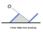
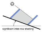
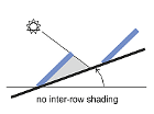
description | Ground terrain characterized by elevation, terrain slope and terrain azimuth. Terrain properties affect the self shading of a fixed angle PV array (note, that 'tilt' and 'row spacing' attributes of PV modules on the pictures below are identical - what is changing is the terrain slope and how it affects the self shading). |


   | |
content | none |
|---|---|
@elevation | optional, meters above the mean see level. If missing, the value will be taken from SRTM terrain database |
@azimuth | optional, orientation of tilted terrain in degrees, 0 for North, 180 for South, clockwise, default is 180, has no effect for the flat terrain (tilt=0) |
@tilt | optional, slope tilt of the terrain in degrees, 0 for flat ground, 90 for vertical surface, default is 0 (flat) |
element name | horizon |
|---|---|
defined in | |
description | User can provide custom skyline for expressing distant or close obstruction features (hills, trees, buildings, poles, etc.) |
content | String of this form: space-delimited list of float number pairs [azimuth in degrees:0-360]:[horizon height in degrees:0-90], Example: "<geo:horizon>0:3.6 123:5.6 359:6</geo:horizon>" |
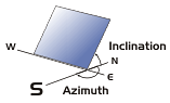
element name | geometry |
|---|---|
defined in | |
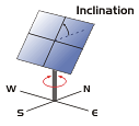
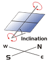
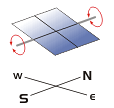
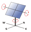
description | Parametrization of PV system mounting type used for calculating GTI and PVOUT. If this element is missing and GTI/PVOUT is requested, flat-lying PV panels are considered (GTI=GHI). Examples: <pv:geometry xsi:type="pv:GeometryFixedOneAngle" azimuth="180" tilt="25"/> <pv:geometry xsi:type="pv:GeometryOneAxisHorizontalNS" rotationLimitEast="-90" rotationLimitWest="90" backTracking="true" azimuth="180"/> <pv:geometry xsi:type="pv:GeometryOneAxisInclinedNS" axisTilt="30" rotationLimitEast="-90" rotationLimitWest="90" backTracking="true" azimuth="180"/> <pv:geometry xsi:type="pv:GeometryOneAxisVertical" tilt="25" rotationLimitEast="-180" rotationLimitWest="180" backTracking="true"/> <pv:geometry xsi:type="pv:GeometryTwoAxisAstronomical" rotationLimitEast="-180" rotationLimitWest="180" tiltLimitMin="10" tiltLimitMax="60" backTracking="true"/> |
content | none |
@type* | required, type of the mounting geometry. Use one from GeometryFixedOneAngle, GeometryOneAxisHorizontalNS, GeometryOneAxisInclinedNS, GeometryOneAxisVertical, GeometryTwoAxisAstronomical, see table below for pictures. |
@azimuth | the value in degrees of a true geographical azimuth (0: north, 90: east, 180: south, 270: west, 360: north --> a compass value) . In the case of 'GeometryFixedOneAngle' the azimuth attribute is required. In the case of two tracker types (GeometryOneAxisHorizontalNS, GeometryOneAxisInclinedNS) the value is the compass value at which the southern end of the tracker axis is oriented. Regardless of the Earth's hemisphere. With trackers, the value is limited to the range from 135 deg. to 225 deg. inclusive, so the deviation from the north-south line is not bigger than 45 degrees. With trackers, the attribute is optional and it defaults to 180 deg. (which means the southern end of the axis faces to geographical south, so the tracker field is aligned with the north-south line which is the optimal solution for most cases). |
@tilt | tilt of panel surface in degrees range (0, 90), 0=horizontal, 90=vertical surface, required for 'GeometryFixedOneAngle' and 'GeometryOneAxisVertical' types |
@axisTilt | optional, default is 30 deg., allowed range is (0, 90). Tilt of rotating inclined axis in degrees, 0 = horizontal, 90 = vertical axis, only applicable for 'GeometryOneAxisInclinedNS', WARNING: if this attribute is missing, the value defaults to 30 degree. |
@rotationLimitEast | optional, for trackers only default values / allowed ranges:
The general rule is: negative values are used for the east side, positive for the west side, the same rule applies for both Earth hemispheres). The value of rotationLimitEast must be smaller or equal than the rotationLimitWest. |
@rotationLimitWest | optional, for trackers only default values / allowed ranges:
The general rule is: negative values are used for the east side, positive for the west side, the same rule applies for both Earth hemispheres). The value of rotationLimitEast must be smaller or equal than the rotationLimitWest. |
@tiltLimitMin | optional, for trackers only Default is 0 deg, allowed range: 0, 90. Used with the horizontal axis of GeometryTwoAxisAstronomical tracker. Limit is defined relative to the horizontal position of the tracking surface (0 deg.). Example: if set as tiltLimitMin="0" and tiltLimitMax="60" - the tracker follows the sun elevation in the range from horizontal position to 60 degree of tilt. The value of tiltLimitMin must be smaller or equal than the tiltLimitMax. |
@tiltLimitMax | optional, for trackers only Default is 90 deg, allowed range: 0, 90. Used with the horizontal axis of GeometryTwoAxisAstronomical tracker. Limit is defined relative to the horizontal position of the tracking surface (0 deg.). Example: if set as tiltLimitMin="0" and tiltLimitMax="60" - the tracker follows the sun elevation in the range from horizontal position to 60 degree of tilt. The value of tiltLimitMin must be smaller or equal than the tiltLimitMax. |
@backTracking | optional boolean value, default is 'false' - tracker moves freely regardless of the neighbors, value is 'true' - tracker moves in the way that it avoids shading from neighboring tracker constructions. |
Table of supported geometries (PV mounting types):
GeometryFixedOneAngle | GeometryOneAxisVertical | GeometryOneAxisInclinedNS | GeometryOneAxisHorizontalNS | GeometryTwoAxisAstronomical |
|---|
 |

 |
 |
 |
 | ||||
|
|
|
|
|
PV system
element name | system |
|---|---|
defined in | |
description | Parametrization of the PV system. Required for simulating PVOUT parameter. |
content | required one <module> element, required one <inverter> element, required one <losses> element, optional one <topology> element, |
@installedPower* | required float value (greater than zero). Total installed DC power of the PV system in kilowatts-peak (kWp). The total PV system rating consists of a summation of the panel ratings measured in STC. |
@installationType | optional, use one from FREE_STANDING (default), ROOF_MOUNTED, BUILDING_INTEGRATED. This property of the PV system helps to estimate how modules are cooled by air. For sloped roof with PV modules on rails tilted at the same angle as the roof choose 'ROOF_MOUNTED' value. For PV modules incorporated into building facade choose 'BUILDING_INTEGRATED' value. This option is considered as the worst ventilated. As the best ventilated option is considered 'FREE_STANDING' installation. This typically means stand-alone installation on tilted racks anchored into the ground. Also choose this option if a PV system is installed on a flat roof. |
@dateStartup | optional string formatted as "yyyy-mm-dd" (example 2015-01-01). Start-up date of the PV system (unpacking of modules). This parameter is used for calculation of degradation of modules caused by aging. If omitted, the degradation is not taken into account. |
@selfShading | optional, default is 'false'. The parameter affects PV power calculation for 'GeometryFixedOneAngle' geometry, then 'GeometryOneAxisInclinedNS' and 'GeometryOneAxisHorizontalNS' trackers if backTracking="false". When 'selfShading' is switched on, the simulated PV power is typically lower comparing to standalone PV construction not affected by shading from its neighbors. With trackers, always switch off 'backTracking' attribute, because the back tracking avoids self-shading. |
element name | module |
|---|---|
defined in | |
description | Parametrization of the PV system modules. Required for simulating PVOUT parameter. All modules in one PV system are considered of the same type. |
content | optional one <degradation> element, optional one <degradationFirstYear> element, optional one <surfaceReflectance> element, optional one <nominalOperatingCellTemp> element, optional one <PmaxCoeff> element |
@type* | required. Enumerated codes for materials used in PV modules. Use 'CSI' for crystalline silicon, 'ASI' for amorphous silicon, 'CDTE' for cadmium telluride, 'CIS' for copper indium selenide. For the estimate of module's surface reflectance we use an approach described here. |
element name | degradation |
|---|---|
defined in | |
description | Estimated annual degradation [%] of rated output power of PV modules. This element is only considered if "dateStartup" attribute of PV system is present. If the element is missing, degradation defaults to 0.5%/year. |
content | required, float number in the range (0, 100), % |
element name | degradationFirstYear |
|---|---|
defined in | |
description | Estimated annual degradation [%] of rated output power of PV modules in the first year of operation. If the element is missing, degradation defaults to 0.8%/year. |
content | required, float number in the range (0, 100), % |
element name | surfaceReflectance |
|---|---|
defined in | |
description | Empirical dimensionless ratio. Typical value 0.12. |
content | required, float number |
element name | nominalOperatingCellTemp |
|---|---|
defined in | |
description | Normal operating cell temperature (NOCT). Float value of the temperature in degrees Celsius of a free standing PV module exposed to irradiance of 800 W/m2 in the ambient air temperature of 20°C and wind speed of 1 m/s. The value is given by manufacturer and for ventilated free-standing PV systems only. If the element is missing, the NOCT value defaults to (based on technology): CSI=46°C |
content | required, float number in degrees Celsius |
element name | PmaxCoeff |
|---|---|
defined in | |
description | Negative percent float value representing the change of PV panel output power for temperatures other than 25°C (decrease of output power with raising temperature). This property is given at the STC by manufacturer. If the element is missing, the PmaxCoeff value defaults to (based on technology): CSI=-0.438%/°C |
content | required, float number, percent per degree Celsius (%/°C) |
element name | inverter |
|---|---|
defined in | |
description | Parametrization of the PV system inverter. Required for simulating PVOUT parameter. All inverters in one PV system are considered of the same type. |
content | optional one <efficiency> element, optional one <limitationACPower> element |
element name | efficiency |
|---|---|
defined in | |
description | Efficiency of the inverter. If the element is missing, the efficiency is given as a constant value of 97.5%. |
@type* | required, concrete type of how efficiency of the inverter should be modeled. Use one from EfficiencyConstant, EfficiencyCurve |
content | required, based on type: EfficiencyConstant: float number, [%]. Value of inverter's efficency known as Euro or CEC (California Energy Commission) efficiency. This value is a calculated weighted efficiency given by manufacturer. It gives a simplified picture about an inverter's, in fact non-linear, performance. Valid range of this value is typically in the range 70%-100%. For better results, it is recommended to provide inverter's efficiency curve. EfficiencyCurve: text value, pairs of kW:percent. Efficiency of inverter is of non-linear nature, so it can be described as simplified curve defined as list of data points. Data point on the curve is defined by coordinates, where the x coordinate is absolute float value of input power in kilowatts (kW) and y coordinate is percent float value of the corresponding inverter's efficiency (%). This parameter accepts string value of this pattern: 'x1:y1 x2:y2 x3:y3 xn:yn'. A dot should be used as decimal separator, white space as a pair delimiter and colon as x:y delimiter. We assume the last point determines the maximum input power of the inverter (with corresponding efficiency). Example of an efficiency curve with the maximum input power of 3 kW is: <pv:efficiency xsi:type="pv:EfficiencyCurve" dataPairs="0:85.6 0.5:96.2 1:98 1.5:97 2:97 2.5:96 3.0:96"/> It is assumed, that one efficiency curve is valid for all inverters of the PV system (their powers are summed). |
element name | limitationACPower |
|---|---|
defined in | |
description | Maximum power accepted by the inverter as AC output. Higher power values are 'clipped'. Clipping refers to the situation where the AC power output of an inverter is limited due to the peak rating of the inverter (the parameter value in kW), even though the additional power may still be available from the solar modules. If you have power factor (PF) and AC limit in kVA available, use this formula: PF * AC_limit_kVA = kW, to obtain the value of this parameter. No default. |
content | required, float number, kilowatts [kW] |
element name | losses |
|---|---|
defined in | |
description | Estimation of various PV losses. |
content | optional one <acLosses> element, optional one <dcLosses> element |
element name | dcLosses |
|---|---|
defined in | |
description | Estimation of power losses on the DC side. If the element is missing, the specific DC losses are estimated by default as: snowPolution: 2.5% cables: 2.0% mismatch: 1.0% |
content | none |
@snowPollution | annual value of estimated dirt and snow losses [%] |
@monthlySnowPollution | Distribution of the 'snowPollution' attribute value into 12 monthly average values. Value of the parameter must consist of 12 percent float values delimited by white space. If this parameter is present, it takes precedence over 'snowPollution' attribute. Example: <pv:dcLosses cables="0.2" mismatch="0.3" monthlySnowPollution="5 5.2 3 1 1 1 1 1 1 1 2 4"/> |
@cables | annual value of estimated DC cabling losses [%] |
@mismatch | annual value of estimated DC mismatch losses [%] |
element name | acLosses |
|---|---|
defined in | |
description | Estimation of power losses on the AC side. If the element is missing, the specific AC losses are estimated by default as: transformer: 1.0% cables: 0.5% |
content | none |
@transformer | annual value of estimated transformer losses [%] |
@cables | annual value of estimated AC cabling losses [%] |
element name | topology |
|---|---|
defined in | |
description | The element is for defining PV plant layout on the ground. The reason is to provide inputs for calculation of self-shading impact on PV power (e.g., how close to each other are PV constructions). |
content | none |
@type* | XML element type, required, concrete type of how topology should be modeled. Use one from TopologyRow (applies for the 'GeometryFixedOneAngle' geometry), TopologyColumn (use for all trackers). It is assumed trackers are spaced equally in both directions (rows and columns) creating a regular grid. |
@relativeSpacing | required, unitless ratio. The attribute specifies the ratio of distance between the neighboring PV table legs and PV table width. Direction of the distance depends on whether topology is specified as TopologyRow or TopologyColumn. See picture below how to calculate the value. |
@type | optional. This parameter estimates a magnitude of loss of PV power when modules are shaded or semi-shaded. The effect depends on wiring interconnections within a module. Shading influence ranges from 0% (no influence) to 100% (full influence) and it is classified into following categories (based on the influence value): PROPORTIONAL = 20% (for a-Si, CdTe and CIS where the loss of generated electricity is proportional to the size of module area in shade) When this attribute is missing, the self-shading influence is estimated to 5%. |
...
Figure: Calculation of relative row spacing value (= x3/x2). :
...
For sub-hourly data the PVOUT value typically represents instantaneous value (a power measured exactly at the given timestamp), so the PVOUT unit will be the kW (or W/m2 in case of irradiation).
...
| Note |
|---|
Timestamps used in the XML response comply with the ISO 8601 standard for date and time representation https://en.wikipedia.org/wiki/ISO_8601. Time stamps are also aware of time zone (offset from UTC). Time zone designators are appended after the the time part of timestamp string. If the time is in UTC (https://en.wikipedia.org/wiki/Coordinated_Universal_Time), Z is added directly after the time without a space. Z is the zone designator for the zero UTC offset e.g., 2017-09-22T01:00:00.000Z . If there is an offset from UTC, this is designated by appending +/-HH:MM after the timestamp string, e.g., 2017-09-22T01:00:00.000-05:00 (UTC-5). |
| Code Block | ||
|---|---|---|
| ||
<?xml version="1.0"?>
<dataDeliveryResponse xmlns="http://geomodel.eu/schema/ws/data" xmlns:ns2="http://geomodel.eu/schema/common/geo">
<site id="demo" lat="48.61259" lng="20.827079">
<metadata>#15 MINUTE VALUES OF SOLAR RADIATION AND METEOROLOGICAL PARAMETERS AND PV OUTPUT
#
#Issued: 2017-09-03 12:40
#
#Latitude: 48.612590
#Longitude: 20.827079
#Elevation: 7.0 m a.s.l.
#http://solargis.info/imaps/#tl=Google:satellite&loc=48.612590,20.827079&z=14
#
#
#Output from the climate database Solargis v2.1.13
#
#Solar radiation data
#Description: data calculated from Meteosat MSG satellite data ((c) 2017 EUMETSAT) and from atmospheric data ((c) 2017 ECMWF and NOAA) by Solargis method
#Summarization type: instantaneous
#Summarization period: 28/04/2014 - 28/04/2014
#Spatial resolution: 250 m
#
#Meteorological data
#Description: spatially disaggregated from CFSR, CFSv2 and GFS ((c) 2017 NOAA) by Solargis method
#Summarization type: interpolated to 15 min
#Summarization period: 28/04/2014 - 28/04/2014
#Spatial resolution: temperature 1 km, other meteorological parameters 33 km to 55 km
#
#Service provider: Solargis s.r.o., M. Marecka 3, Bratislava, Slovakia
#Company ID: 45 354 766, VAT Number: SK2022962766
#Registration: Business register, District Court Bratislava I, Section Sro, File 62765/B
#http://solargis.com, contact@solargis.com
#
#Disclaimer:
#Considering the nature of climate fluctuations, interannual and long-term changes, as well as the uncertainty of measurements and calculations, Solargis s.r.o. cannot take full guarantee of the accuracy of estimates. The maximum possible has been done for the assessment of climate conditions based on the best available data, software and knowledge. Solargis s.r.o. shall not be liable for any direct, incidental, consequential, indirect or punitive damages arising or alleged to have arisen out of use of the provided data. Solargis is a trade mark of Solargis s.r.o.
#
#Copyright (c) 2017 Solargis s.r.o.
#
#
#Columns:
#Date - Date of measurement, format DD.MM.YYYY
#Time - Time of measurement, time reference UTC+2, time step 15 min, time format HH:MM
#GHI - Global horizontal irradiance [W/m2], no data value -9
#GTI - Global tilted irradiance [W/m2] (fixed inclination: 25 deg. azimuth: 180 deg.), no data value -9
#TEMP - Air temperature at 2 m [deg. C]
#WS - Wind speed at 10 m [m/s]
#WD - Wind direction [deg.]
#AP - Atmospheric pressure [hPa]_
#RH - Relative humidity [%]
#PVOUT - PV output [kW]
#
#Data:
Date;Time;GHI;GTI;TEMP;WS;WD;AP;RH;PVOUT</metadata>
<columns>GHI GTI TEMP WS WD AP RH PVOUT</columns>
....
<row dateTime="2014-04-28T05:11:00.000+02:00" values="0.0 0.0 10.2 1.9 10.0 1005.4 81.2 0.0"/>
<row dateTime="2014-04-28T05:26:00.000+02:00" values="5.0 5.0 10.4 1.9 10.0 1005.4 80.3 0.0"/>
<row dateTime="2014-04-28T05:41:00.000+02:00" values="12.0 11.0 10.6 1.9 10.0 1005.3 79.5 2.85"/>
<row dateTime="2014-04-28T05:56:00.000+02:00" values="25.0 25.0 10.9 2.2 10.0 1005.3 78.7 11.936"/>
<row dateTime="2014-04-28T06:11:00.000+02:00" values="38.0 37.0 11.2 2.2 10.0 1005.2 77.9 21.25"/>
<row dateTime="2014-04-28T06:26:00.000+02:00" values="102.0 70.0 11.9 2.2 10.0 1005.1 76.5 38.582"/>
<row dateTime="2014-04-28T06:41:00.000+02:00" values="144.0 112.0 12.7 2.2 10.0 1005.0 75.0 68.925"/>
<row dateTime="2014-04-28T06:56:00.000+02:00" values="183.0 156.0 13.4 2.1 9.0 1004.9 73.5 106.197"/>
<row dateTime="2014-04-28T07:11:00.000+02:00" values="223.0 202.0 14.2 2.1 9.0 1004.8 72.1 150.239"/>
<row dateTime="2014-04-28T07:26:00.000+02:00" values="265.0 252.0 14.8 2.1 9.0 1004.7 71.2 197.703"/>
<row dateTime="2014-04-28T07:41:00.000+02:00" values="308.0 304.0 15.3 2.1 9.0 1004.7 70.3 248.14"/>
<row dateTime="2014-04-28T07:56:00.000+02:00" values="354.0 359.0 15.8 1.7 8.0 1004.6 69.4 301.096"/>
<row dateTime="2014-04-28T08:11:00.000+02:00" values="403.0 420.0 16.4 1.7 8.0 1004.6 68.4 357.374"/>
<row dateTime="2014-04-28T08:26:00.000+02:00" values="450.0 479.0 16.9 1.7 8.0 1004.7 66.0 411.019"/>
<row dateTime="2014-04-28T08:41:00.000+02:00" values="497.0 544.0 17.5 1.7 8.0 1004.8 63.5 468.12"/>
<row dateTime="2014-04-28T08:56:00.000+02:00" values="539.0 599.0 18.0 1.8 26.0 1004.8 61.0 515.073"/>
...
<row dateTime="2014-04-28T23:41:00.000+02:00" values="0.0 0.0 14.1 2.9 353.0 1004.8 93.3 0.0"/>
<row dateTime="2014-04-28T23:56:00.000+02:00" values="0.0 0.0 14.0 2.8 354.0 1004.8 93.3 0.0"/>
</site>
</dataDeliveryResponse> |
Push data delivery
CSV request examples
...